Safety measures concerning the Coronavirus COVID-19. Read more about the measures.

x

Annex to Chapter 1

Online annexes to Chapter 1 of the Euro Area Stability Watch present the data sources, analytical frameworks, and methodologies supporting the chapter’s risk assessment. They are organised in line with the chapter structure, covering the technical underpinnings of the boxes, the design of the adverse macroeconomic and fiscal scenarios, and key indicators, alongside additional analyses and robustness checks. 

A1 Data and methodological supplement to Box 1.1

This annex provides details on the methodology underlying the analysis presented in Box 1.1. A large language model extracts structured, market-relevant news indicators from daily expert commentary, which then feed into a factor-augmented event study regression to quantify how different types of news move financial variables.  

A1.1 Large language model-based extraction of news dummies

Text data source and news extraction pipeline

The text corpus for our analysis is a daily commentary available since September 2018 and produced by experts from the International Monetary Fund's Monetary and Capital Markets Department (the Global Markets Monitor). The large language model analyses each report in the sample and extracts a small set of news items, which were reported as relevant for equity and government bond price movements, respectively. Specifically, each day’s Global Markets Monitor report is parsed by the model with a prompt that instructs it to identify the distinct market-moving news and events discussed in the commentary and assign each item to one of 15 pre-defined, economically interpretable categories following Baker et al. (2025). In a second step, for our regression analysis, we further aggregate the original classifications of Baker et al. (2025) into five headline categories as follows (original categories in brackets):  

  1. Global markets (commodities, foreign markets)  
  2. Macroeconomy (macroeconomic news and outlook, corporate earnings and outlook, other non-policy)
  3. Monetary policy
  4. Fiscal and structural policy (government spending, taxes, exchange rate policy, capital controls, international trade policy, regulation, elections and political transitions, other policy)
  5. Conflicts and security (sovereign military and security actions, terrorist attacks and large-scale violence by non-state actors) 

From news items to daily news dummies

For each category, the large language model analysis generates two daily `news dummies’ (one for risk-free yields and one for equities) that take the value of 1 if the commentary for day 𝑡 contains at least one event of the category that is associated with movements in bond or equity prices. The two resulting sparse matrices of category-by-day dummies then feed into the factor-augmented event study regression (denoted \[ d_1^{news} \] and \[ d_2^{news} \] in the equation below). 

A1.2 Factor-augmented event-study model with latent news factors

Data

We combine daily financial-market data with macroeconomic release surprises, monetary policy surprises, and the news measures outlined in Section A1.1. Euro area risk-free yields are proxied by the German yield curve: the first and fourth Euribor futures and 2-, 5-, 10-, and 30-year Bund futures (Gürkaynak et al., 2022). Other variables include the EUROSTOXX 50, the VSTOXX index, aggregate corporate spreads (AAA, BBB, high-yield), and the euro area TED spread (3-month EURIBOR minus 3-month Bund yield). Since euro area macroeconomic data surprises are conceptually largely unavailable due to earlier country-specific releases and known country weights, we use 13 important indicators for the German economy, where surprises are defined as the released value minus the median expectation of survey participants. The data were obtained from Bloomberg. Monetary policy surprises comprise the monetary policy and central bank information components for the European Central Bank and the Federal Reserve (Jarocinski and Karadi, 2020), with the latter being shifted by one day (t+1) to account for time zone differences.


Econometric model

The decompositions shown in Box 1.1 are based on the following specification. The model is motivated by Gürkaynak et al. (2020), extending their analysis in terms of both dependent and explanatory variables. Our specification decomposes (de-meaned) daily changes in the yields of (risk-free) government bonds at different maturities (\[ r_t \] with dimension \[ N_1 \] × 1) and the other market-based (risk) measures (𝜎𝑡 with dimension \[ N_2 \] × 1) as follows:

\[ \begin{bmatrix} r_t \\ \sigma_t \end{bmatrix} = \begin{bmatrix} \beta^r \\ \beta^\sigma \end{bmatrix} s_t + \begin{bmatrix} \gamma^r \\ \gamma^\sigma \end{bmatrix} d_t^s f_{1,t} + \begin{bmatrix} \delta_1^r \\ \delta_1^\sigma \end{bmatrix} \left( d_{1,t}^{news} \odot f_{2,t} \right) + \begin{bmatrix} \mathbf{0} \\ \delta_2^\sigma \end{bmatrix} \left( d_{2,t}^{news} \odot f_{3,t} \right) + \varepsilon_t \\[1em] f_{1,t} \sim N(0,1), \quad f_{2,t} \sim N\left(\mathbf{0}, I_{K_2}\right), \quad f_{3,t} \sim N\left(\mathbf{0}, I_{K_2}\right), \quad \varepsilon_t \sim N(\mathbf{0}, \Sigma) \]

with t = 1, …, \[ T \], i = 1, …, \[ N \], \[ N = N_1 + N_2 \], and where \[ s_t \] is a (\[ K_1 \] × 1) vector of observed data release surprises, \[ d^s_t \] is a dummy vector for release days (one if any of the indicators in s was published on day t), and \[ d_{1,t}^{news} \],t and \[ d_{2,t}^{news} \] are (K2 × 1) dummy matrices for bond and equity market-relevant news, respectively. The unobserved data release factor \[ f_{1,t} \] and the (\[ K_2 \] × 1) unobserved news factors \[ f_{2,t} \] and \[ f_{3,t} \] are assumed normally distributed with unit variance to identify their scales. The flexible two-factor structure for the news components is motivated by recent analyses suggesting that aggregate financial conditions can be characterised by two distinct factors, one capturing dynamics in risk-free yields and the other capturing financial risk (Lombardi et al., 2025). \[ \beta^r \], \[ \beta^\sigma \], \[ \gamma^r \], \[ \gamma^\sigma \], \[ δ^r_1 \],\[ δ^σ_1 \], and \[ δ^σ_2 \] are coefficient matrices of corresponding dimensions. Lastly, \[ \varepsilon_t \] is the error term, with diagonal covariance matrix Σ. The model is estimated with a Bayesian approach (Gibbs sampling), using relatively uninformative prior distributions. The contribution of data surprises shown in the charts includes both observed and unobserved data release surprises, with the latter being captured through \[ f_{1} \]. Finally, the contributions of the news categories for the non-yield variables reflect the combined impact of \[ f_{2} \] and \[ f_{3} \]. 

A1.3 References

Baker, S. R., N. Bloom, S. J. Davis, and M. Sammon. What triggers stock market jumps?, mimeo, 2025.

Gürkaynak, R. S., B. Kisacikoglu, and J. H. Wright. Missing events in event studies: Identifying the effects of partially measured news surprises, American Economic Review, 110(12):3871–3912, 2020.

Gürkaynak, R. S., M. Kerssenfischer, B. Kisacikoglu, and J. H. Wright. News and noise shaping international yield curves, mimeo, 2022.

Jarocinski, M. and P. Karadi. Deconstructing monetary policy surprises: the role of information shocks, American Economic Journal: Macroeconomics, 12(2):1–43, 2020.

Lombardi, M. J., C. Manea, and A. Schrimpf. Financial conditions and the macroeconomy: a two-factor view, BIS Working Papers, 1272, Bank for International Settlements, 2025.


A2 Data and methodological supplement to Box 1.2

This annex provides details on the methodology underlying the analysis presented in Box 1.2. It outlines the data and empirical framework used to estimate the effects of geopolitical risk and financial uncertainty shocks on foreign investor inflows into euro area and United States (US) government debt securities from January 1999 to December 2024. 

A2.1 Shocks

We use the global geopolitical risk (GPR) index of Caldara and Iacoviello (2022) as our main measure of adverse geopolitical episodes. The index is constructed as the share of newspaper articles containing GPR-related keywords in major Anglo‑American newspapers, relative to the total number of published articles. It provides a high-frequency, text-based measure of global geopolitical tensions. 

In addition, we include the VIX index (a measure of US stock market volatility) to proxy for global financial market uncertainty. While related, GPR and financial uncertainty are conceptually different. The former reflects geopolitical events and tensions, whereas the latter captures broader market volatility and risk sentiment. Caldara and Iacoviello (2022) show that the GPR index displays substantial independent variation relative to both the VIX and the news-based Economic Policy Uncertainty index of Baker, Bloom, and Davis (2016). This allows us to study these two distinct sources of shocks separately. 

All shock variables are standardised to have zero mean and unit variance. Therefore, the estimated coefficients can be interpreted as the response to a one standard deviation shock. To allow for nonlinear effects, we further define high-risk periods as observations in which the shock exceeds its 90th percentile. 

A2.2 Monthly portfolio debt liability flows into government securities

Data on non‑euro area investors’ net purchases of euro area government securities are sourced from the European Central Bank (ECB) balance of payments statistics dataset and are available at monthly frequency from 2008. Data coverage includes both short‑ and long‑term instruments. To ensure comparability with the US analysis, euro area flows are extended back to 1999. For the 1999–2007 period, flows are constructed by aggregating non‑resident net purchases for euro area countries with available data, using ECB balance of payment statistics and national central bank sources. These imputed flows before 2008 include transactions by investors resident in other euro area countries. Results based solely on reported ECB balance of payment statistics from 2008 onward are qualitatively similar, and including intra‑euro area flows does not materially affect the findings over the common sample period 2008–2024. 

Monthly data on foreign investors’ net purchases of US government securities are sourced from the Treasury International Capital (TIC) system. As recommended by Bertaut and Judson (2025), reported TIC data are used from 2023 onward, while earlier flows are based on valuation-adjusted estimates from Bertaut and Tryon (2007) and Bertaut and Judson (2014, 2022), using information from the TIC Survey of Long-Term Securities. US government securities include both Treasury and agency securities. Long‑term instruments (above one year) are drawn from the valuation‑adjusted datasets, while short‑term instruments are directly sourced from TIC data. Compared with the euro area data, the US data provide greater granularity along both the counterpart-sector and counterpart-country dimensions. This enables distinguishing between foreign official investors (primarily foreign central banks) and foreign private investors, and, within the latter group, between investors resident inside and outside the euro area.  

Flow data are scaled by one-year-lagged annual gross domestic product (GDP). The analysis relies on monthly flow data without any further transformation. A local projection specification, discussed in detail below, is then used to estimate cumulative flow responses to shocks. Results are robust to using three-month moving averages, which yields smoother impulse responses. 

A2.3 Local projections framework

Our empirical strategy examines how foreign investors’ flows into government securities respond to GPR and financial-market uncertainty shocks using monthly local projections in the style of Jordá (2005). The analysis is conducted separately for the US and the euro area. For each forecast horizon h=0, 1, 2,…, 12, we estimate:

\[ \sum_{j=0}^{h} y_{t+j} = \alpha^{(h)} + \beta_1^{(h)} shock_t + \beta_2^{(h)}\left(shock_t \times \mathbb{1}(shock_t > q_{0.9})\right) + \beta_3^{(h)}\left(\mathbb{1}(shock_t > q_{0.9})\right) + \\ \sum_{s=1}^{p} \delta_s^{(h)}(y_{t-s}) + \sum_{s=1}^{k} \gamma_s^{(h)} Z_{t-s} + \varepsilon_{t+h} \]

The dependent variable y is monthly portfolio liability flows into government debt securities, expressed as a share of annual GDP in period t−12 (same scaling for each h). The variable shock corresponds to either GPR or financial-market volatility (measured by the VIX), both standardised. To capture nonlinear effects, we interact the shock with an indicator for high-risk periods, defined as observations above the 90th percentile of the shock distribution.

The vector Z includes a set of lagged control variables (including lags of the shock) capturing global financial conditions and macro-financial characteristics, considered as push and pull factors of capital flows, respectively. The specification differs slightly between the euro area and the US to reflect relevant market structures. For euro area (US) specifications, the baseline controls include VIX, the STOXX 600 index (S&P 500 index), Brent oil prices (WTI oil prices), the US NFCI, and 3-month EURIBOR (3-month US government yields). All controls, except the VIX, are expressed in first differences to address non-stationarity. While all control variables are included with two lags, the dependent variable is included with up to 12 lags to account for persistence in capital flows; results are robust to alternative lag lengths of two and six.

The impulse response functions are constructed from the sequence of estimated coefficients \[ \left\{\beta_1^{(h)}\right\}_{h=0}^{H} \]​, which tracks the dynamic cumulative response of capital flows to shocks during normal periods. Specifically, the additional effect during high-risk episodes is captured by the sequence \[ \left\{\beta_2^{(h)}\right\}_{h=0}^{H} \], which measures how the cumulative response of capital flows differs when shocks occur in periods of heightened geopolitical or financial stress.

A2.4 Supplementary results 

We also employ a euro area-specific geopolitical risk measure (hereafter GPREA8) designed to capture episodes in which geopolitical tensions are directly centred on the euro area. Caldara and Iacoviello (2022) provide country-specific GPR indices based on articles combining geopolitical-risk keywords with country identifiers; we construct GPREA8 as the simple average of eight euro area country indices. It complements the global GPR index by isolating regionally relevant geopolitical shocks that may have different implications for capital flows given differences in geographical proximity and exposure to geopolitical events. As illustrated in Figure A2.1, GPR and GPREA8 do not always peak in the same periods; and even when their peaks coincide, they often differ in intensity, reflecting differences in the underlying events they capture. 
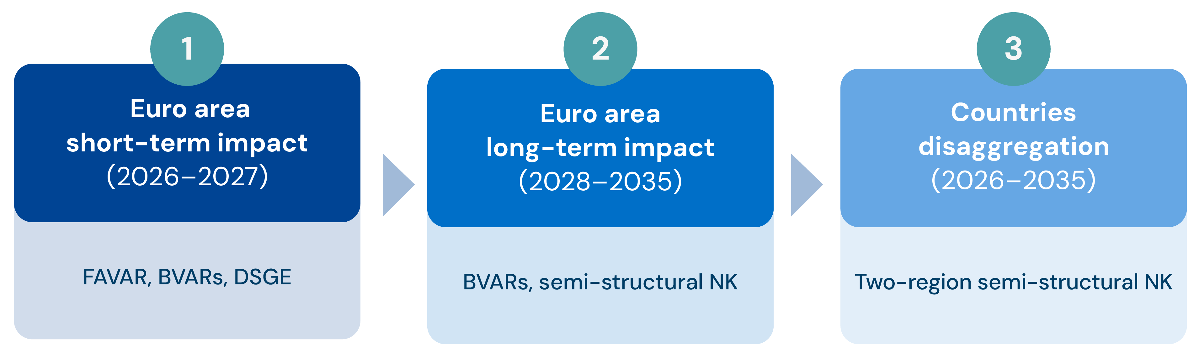
Figure A2.1

Standardised GPR and GPREA8 indices

(January 1999 to December 2025)

Note: Standardised GPR and GPREA8 indices, together with the months in which each index exceeds its 90th
percentile.
Source: ESM calculations based on Caldara and Iacoviello (2022) data

Interestingly, when extreme geopolitical tensions are closely linked to the euro area, foreign demand for US sovereigns reasserts itself. Using GPREA8, results show that periods of elevated geopolitical tensions centred on the euro area (such as the Russian invasion of Ukraine), prompt short-lived inflows into US Treasuries from foreign investors, including those of the euro area, peaking after a quarter (Figure A2.2). At the same time, foreign demand for euro area sovereign debt remains resilient, with no evidence of reversal and, if anything, a mildly positive response in the aftermath of such shocks. This reinforces our main finding that euro area sovereign debt remains resilient even during episodes of high geopolitical stress concentrated within the region.  

Figure A2.2

Flows into government bonds after euro area-specific GPR shocks

Notes: Cumulative impulse responses following a one standard deviation shock in the euro area GPR (GPREA8), in months when GPREA8>90th percentile. Shaded areas: 68% confidence intervals.
Source: ESM calculations

A2.5 References 

Caldara, D. and M. Iacoviello (2022). Measuring geopolitical risk. American Economic Review, 112(4), 1194–1225. 

Baker, S. R., N. Bloom, and S.J. Davis (2016). Measuring economic policy uncertainty. Quarterly Journal of Economics, 131(4), 1593–1636.

Bertaut, C. C. and R. W. Tryon (2007). Monthly estimates of U.S. cross-border securities positions. Federal Reserve Board International Finance Discussion Papers, No. 2007-910. 

Bertaut, C. C. and R. Judson (2014). Estimating U.S. cross-border securities positions: new data and new methods. Federal Reserve Board International Finance Discussion Papers, No. 2014-1113. 

Bertaut, C. C., and R. Judson (2022). Estimating U.S. cross-border securities flows: ten years of the TIC SLT. Federal Reserve Board FEDS Notes.

Bertaut, C. C., and R. Judson (2025). Measuring U.S. cross-border securities flows: out with the old, in with the new. Federal Reserve Board FEDS Notes.

Jordà, Ò. (2005). Estimation and inference of impulse responses by local projections. American Economic Review, 95(1), 161–182. 

A3 Data and methodological supplement to Box 1.3

This annex provides details on the data and empirical approach used to estimate the effects of the ‘new geopolitical regime’ (since the outbreak of the Russia-Ukraine war) on banks’ lending dynamics, conditional on the level of banks’ sovereign exposures.  

A3.1 Data 

The dataset is an unbalanced panel of 82 banks from 18 euro area countries that spans between Q4 2019 and Q4 2025 at quarterly frequency. Data come from the Transparency Exercise of the European Banking Authority and are merged with macro-financial variables.  

A3.2 Methodology

To estimate the effect of the ‘new regime’ on bank lending – conditional on banks’ sovereign exposures – we employ the local projections method (Jordá, 2005) and estimate the following regression: 

\[ \ln(\text{Loans}_{b,t+h}) - \ln(\text{Loans}_{b,t-1}) = \alpha + \beta_{1,h}\,\text{new regime} + \beta_{2,h}\,\text{sovereign exposures}/TA_{b,t-1} \\ + \beta_{3,h}\,\text{new regime} \times \text{sovereign exposures}/TA_{b,t-1} + \beta_{4,h}\,\text{Controls}_{b,t-1} + \delta_{b,h} + \varepsilon_{b,t+h} \]

Here, Ln(Loansb,t+h)Ln(Loansb,t1) is the log difference of loans of bank b between quarter t1 and t+h, with h=0,1,8. Specifically, we consider loans to energy-intensive sectors (mining, manufacturing, transport, and water supply) and loans to non-energy-intensive sectors as identified by the European Systemic Risk Board (2026).

represents a dummy that assumes the value of 1 from Q2 2022 onwards, corresponding to the quarter after the start of the Russia-Ukraine war, and 0 otherwise. Sovereign exposures/TAb,t1 captures the share of each bank's sovereign exposures (loans and bonds) over total assets. The key term of interest is β3,h (i.e. the interaction new regime×sovereign exposures/TAb,t1), which measures the differential effect of sovereign exposures on bank lending between the ‘old regime’ and the ‘new regime’.

Controlsb,t1is a vector of lagged financial sector and macroeconomic controls. It includes a Covid-19 dummy (dummy=1 for 2020), CET1 ratio (capital position of bank), stage 2 ratio (loans classified as stage 2 over total loans), return on assets, cash ratio (cash over assets), non-bank financial institution asset growth (quarter-on-quarter growth in assets of the non-bank financial institution sector), quarter-on-quarter gross domestic product growth, quarter-on-quarter changes in Euribor, government debt growth (quarter-on-quarter growth rate of government debt) and European Central Bank asset growth (quarter-on-quarter growth of bank's balance sheet). δb,h is bank fixed effects and εb,t+h the error term. Standard errors are clustered at the bank level.

A3.3 References

European Systemic Risk Board (2026), Financial stability risks from geoeconomic fragmentation, January 2026.  

Jordà, Ò. (2005), Estimation and Inference of Impulse Responses by Local Projections, American Economic Review, 95(1), 161–182. 

A4 Data and methodological supplement to Box 1.4

This annex provides details on the data and implementation of the granular instrumental variables (GIV) estimation used to determine the impact of aggregate investor demand shocks on sovereign yield spreads presented in Box 1.4.

A4.1 Granular instrumental variables

While derivations and discussions are provided in Gabaix and Koijen (2021, 2022, 2024), the GIV approach requires modelling choices specific to the application at hand. Refinements to the GIV method create a range of possibilities for construction of the instruments. Specific choices for the results presented in Box 1.4 are outlined below.

Isolating the causal relationship between bond flows and yield movements is challenging due to the endogeneity of bond supply and demand. Within a demand system-based asset pricing framework, the GIV approach addresses this issue by constructing an exogenous instrument Zt from a weighted sum of idiosyncratic shocks uit to different investor groups. Because these shocks ui,t are exogenous investor-specific flows, they are orthogonal to common macroeconomic factors and aggregate market movements, while remaining correlated with the yields. Thus, considering N different investor groups with time-varying market shares Si,t, the GIV instrument is defined as: 

\[ z_t = \sum_{i=1}^{N} S_{i,t-1}\, u_{i,t} \]

Given the instrument z_t, the price impact captured via the change in the spreads Δs_t (vis-à-vis German Bunds) can then consistently be estimated using the regression:

\[ \Delta s_t = c + M z_t + \lambda'\eta_t + \varepsilon_t \]

where M denotes the impact on the spreads, zt is the GIV instrument, and ηt denotes a vector of observed and latent common factors \[ \eta_t = (\eta_t^o,\ \eta_t^l) \], such as macroeconomic conditions or global uncertainty. However, as investor-specific shocks ui,t and latent controls \[ \eta_t^l \] are unobserved, they need to be estimated from data to construct the instrument.

To take heterogeneity across different investor groups into account, we use precision weights: 

\[ E_i = \frac{\bar{\sigma}_{u_i}^{-2}}{\sum_{i=1,\ldots,N} \bar{\sigma}_{u_i}^{-2}} \]

where σ̄ui = max(σui, median(σui)) and σui is the standard deviation of uit computed along the time dimension1. The algorithm cycles through three steps2

  1. Estimate weighted panel regression including observed controls and fixed effects using Ei as regression weights to obtain first stage residuals Δq̌i,t:
    \[ \Delta q_{i,t} = \alpha_i + \gamma'\eta_t^o + \Delta\check{q}_{i,t} \]
  2. Perform principal component analysis on precision-weighted residuals \[ E_i^{\frac{1}{2}} \Delta \check{q}_{i,t} \] to recover latent factors \[ \eta_t^l \] given by the principal components.

  3. Run ordinary least squares regression of common factors \[ \eta_t^l \] on first stage residuals Δq̌i,t: to estimate investor-specific shocks ǔi,t  and update precision weights σ̄ui, and iterate again, where:

\[ \Delta\check{q}_{i,t} = \beta'\eta_t^l + \check{u}_{i,t} \]


Once we have obtained estimates \[ ǔ_{ji,t} \] for each country, we construct the GIV instrument as:

\[ z_{j,t} = \sum_{i=1}^{N} S_{ji,t-1}\, \hat{u}_{ji,t} \]

and collect the recovered latent factors \[ η_t^l \] as controls in the main regression. Once the instruments are obtained for each country in a group, the impact effect is estimated running the group-specific panel regression

\[ \Delta s_t = c + M z_{j,t} + \lambda'\eta_t + \varepsilon_t \]

using the observed and recovered unobserved factors for each country group as controls.
Similarly, we estimate the panel local projections for each country group as follows:

\[ s_{t+h} - s_{t-1} = c_h + M_h z_{j,t} + \lambda_h'\eta_t + \varepsilon_{t+h} \]

We specify three iterations as no significant changes of the precision weights are apparent, suggesting convergence of the algorithm. The regression includes the same set of observed factors to \[ \eta_t^0 \] as Chaudhary et al. (2025) and one additional latent factor \[ \eta_t^l \]obtained from the principal component analysis in step 2.

A4.2  Data

Price sensitivities are measured using 10‑year sovereign yields, obtained from Bloomberg, consistent with an average residual maturity of around 7.5 years over the sample period. 

The estimation is based on quarterly data on investor shares and flows. The sample spans Q4 2014–Q4 2025 and compiles estimates of investor holdings at market value, together with quarterly transactions in debt securities issued by the general government. The data are compiled from several sources, including the European Central Bank (ECB)’s quarterly sector accounts (QSA), securities holdings statistics (SHS), and securities holdings statistics by sector (SHSS), data on the Eurosystem’s asset purchase programmes, the International Monetary Fund’s International Financial Statistics and Eurostat’s balance of payments statistics. 

Data compilation inevitably relies on assumptions. Notably, non-euro area holdings are computed as a residual, while investor flows (net purchases) prior to 2021 – when ECB SHSS data become available – are inferred from valuation-adjusted changes in holdings. Hence, any measurement limitations affecting euro area investor coverage and valuation adjustments are reflected in the residual non-euro area category.

Specifically, the primary data source is the ECB’s QSA which reports, for each country, government debt securities holdings and net transactions for all investors, including a breakdown of domestic investors by sector and a single aggregate category for non-resident investors. For several countries, data on domestic central bank holdings are missing for some periods; coverage is therefore extended using the International Monetary Fund’s International Financial Statistics series on gross claims of monetary authorities on general government at market value. 

A second key source is the ECB’s SHSS, which provides, for each country, a sectoral breakdown of holdings and transactions for euro area investors. SHSS data are available from Q1 2021. Coverage is extended back to 2014 using the discontinued SHS dataset, which reports holdings at market value but not flows. Flows are therefore approximated using changes in holdings, adjusted for valuation effects. Investor-specific valuation changes are computed using QSA data for domestic investors, assuming that valuation effects are comparable across domestic and other euro area investors. As the SHS dataset does not provide a series for Eurosystem holdings, the SHSS coverage is extended using constructed series on stocks and flows implied by asset purchase programmes (securities markets programme, public sector purchase programme, and pandemic emergency purchase programme).

Overall, total holdings are taken from QSA data, with domestic and sectoral breakdowns based on QSA, euro area investor breakdowns based on SHSS, and non‑euro area holdings calculated as a residual. 

For the analysis, euro area countries are classified into two groups based on their latest share of non‑euro area investors, distinguishing five countries with relatively high non‑euro area investor shares and four countries with a more euro area‑dominated investor base (Figure A4.1, panel a). Over the sample period, non‑euro area investor shares average around 31% in the first group and 14% in the second. As regards euro area investors, insurance corporations and pension funds are also more prominent in the first group, whereas the Eurosystem, banks and households account for larger shares in the second group (Figure A4.1, panel b).

  • 1

    The floor on the median precision weight prevents investor groups with very stable flows from playing too extreme a role in the weighted regression.

  • 2

    For notational simplicity we drop the country-specific index j of relevant variables in the exposition of the GIV iterations.

Figure A4.1

A heterogeneous investor base

a)
Non-euro area investor share by country, Q4 2025
(sector market shares, in % of total government debt securities)
b)
Sectoral holdings shares across the two groups of countries
(sector market shares, in % of total government debt securities)

Notes: Panel a) shows estimates of the share of euro area government debt securities held by non‑euro area investors, by country, as of end‑2025. Panel b) presents the sectoral composition of the investor base for two groups of countries, constructed based on their non‑euro area investor shares. The sample comprises nine euro area countries for which data are available prior to the start of the ECB’s quantitative easing: Austria, Belgium, Finland, France, Ireland, Italy, Netherlands, Portugal, and Spain. Germany is not part of either group, as the estimation relies on spreads relative to German Bunds.
Source: ESM calculations based on ECB, Eurostat, and International Monetary Fund data

A4.3  References

Gabaix, X. and R. Koijen (2024). Granular Instrumental Variables. Journal of Political Economy. 123(7), 2274-2303.

Gabaix, X. and R. Koijen (2021). In Search of the Origins of Financial Fluctuations:
The Inelastic Markets Hypothesis. NBER Working Paper, No. w28967.

Chaudhary, M., J. Z. Fu, and H. Zhou (2024). Anatomy of the Treasury Market: Who Moves Yields?. Olin Business School Center for Finance & Accounting Research Paper, No. 2024/14.


A5  Data and methodological supplement to Box 1.5

Results of the ESM Sovereign Sentiment Survey are based on a survey of 31 financial market participants active in euro area sovereign bond markets, conducted between 27 March and 17 April 2026. The sample includes issuers (debt management offices and treasuries), intermediaries, and investors. Sample euro area growth (1.0% median, 1.1% average) and euro area inflation (2.9% average, 3.0% median) expectations over the next 12 months are in line with market consensus; recession probability for the euro area (30% average, 33% median) is above consensus. In addition to the survey, structured interviews were conducted with 18 market participants in April 2026. The survey will be repeated twice a year from now on (Q2 and Q4). 

Figure A5.1

Sentiment towards euro area sovereign bonds

a)
Sentiment towards euro area sovereign bonds 
(share of respondents, in %)
b)
Views on euro area sovereign bond spread levels
(share of respondents, in %)

Note: Spreads between 10-year euro area sovereign bonds and 10-year German sovereign bonds.
Source: ESM Sovereign Sentiment Survey, Q2 2026

Figure A5.2

Euro area interest rates expectations

a)
European Central Bank policy rate expectations
(basis point change exp. over 12 months)
b)
10-year Bund yield level expected in 12 months
(share of respondents, in %)

Note: "bps" stands for basis points.
Source: ESM Sovereign Sentiment Survey, Q2 2026

Figure A5.3

Swap spread and maturity expectations

a)
EUR swap spread level expected in 12 months
(share of respondents, in %)
b)
Average maturity of euro area sovereign issuance over 12 months
(share of respondents, in %)

Notes: Swap spread defined as EUR swap rate less German bond yield. "bps" stands for basis points.
Source: ESM Sovereign Sentiment Survey, Q2 2026

Figure A5.4

Liquidity and financial stability

a)
Liquidity in euro area secondary sovereign bond markets
(share of respondents, in %)
b)
Probability of major financial stability event over next 12 months
(share of respondents, in %)

Source: ESM Sovereign Sentiment Survey, Q2 2026

Figure A5.5

Consequences of adverse events for euro area

a)
Expected euro area sovereign spread reaction to adverse events
(share of respondents, in %)
b)
Consequences of Iran war for euro area sovereign bond markets and economy
(share of respondents, in %)

Source: ESM Sovereign Sentiment Survey, Q2 2026

Figure A5.6

Euro area sovereign bond issuance

a)
Absorption of euro area sovereign bond net issuance
(share of respondents, in %)
b)
Relevance of permanent European Union safe asset for euro area capital markets
(share of respondents, in %)

Source: ESM Sovereign Sentiment Survey, Q2 2026

Figure A5.7

Euro area assets in an international context

a)
Necessary factors to achieve foreign capital inflows into euro area
(share of respondents, in %)
b)
Direction of EUR/USD exchange rate in 12 months
(share of respondents, in %)

Note: SIU stands for savings and investments union. BU stands for banking union.
Source: ESM Sovereign Sentiment Survey, Q2 2026

A6  Methodological notes on the macroeconomic adverse scenario

A6.1  Overview of the modelling framework

This annex describes the framework used to design and quantify the adverse macroeconomic scenario underpinning the risk assessment in Chapter 1. It documents the modelling toolkit, identification strategies, and calibration assumptions used to translate the underlying risk narrative into a consistent set of macroeconomic projections. 

The scenario is constructed relative to a baseline consistent with the European Commission’s spring 2026 economic forecast, which sets the starting point for all variables. A no-policy-change assumption is imposed, whereby neither monetary nor discretionary fiscal policy respond to the materialisation of adverse shocks beyond what is already embedded in the baseline or implied by automatic stabilisers. As a result, the scenario isolates the macroeconomic effects of the identified risk factors. 

The modelling strategy follows a top-down, multi-layered approach. The adverse scenario is developed first at the euro area level and subsequently translated into country-specific projections, ensuring consistency between aggregate and national outcomes. The scenario reflects the joint materialisation of the three risk layers discussed in Chapter 1: persistently high geopolitical tensions and energy prices, a repricing of financial assets of the United States (US), and second-round effects on inflation. Given the multi-dimensional nature of the risks considered, the framework relies on a set of complementary models. Each model captures a specific risk layer or transmission channel, rather than a one-size-fits-all model. Their outputs are combined to derive a single internally consistent macroeconomic path. 

The framework proceeds in three main steps (Figure A6.1):  

  1. First, the short-term euro area impact (2026–2027) is quantified. This step translates the identified risk layers of the adverse scenario (rise in geopolitical risks and energy prices, repricing of US assets, and second-round effects on inflation) into macroeconomic outcomes. To calibrate the different shocks and capture the relevant transmission channels, the analysis draws on a combination of empirical and structural models, including factor-augmented vector autoregressions (FAVAR), Bayesian vector autoregressions (BVAR), and dynamic stochastic general equilibrium (DSGE) models. The resulting effects on growth and inflation reflect the joint contribution of the impacts of each of three risk layers. 
  2. Second, the scenario is extended to the medium to long term (2028–2035). Persistent geopolitical tensions and higher energy prices are assumed to weigh on productivity and external competitiveness, generating scarring effects on output. These channels are quantified using empirical (BVAR) and semi-structural models to derive a medium- to long-term trajectory for gross domestic product (GDP) consistent with the adverse environment described above. Other shocks, particularly those related to US asset repricing, are assumed to have temporary effects and therefore do not materially affect long-term dynamics. 
  3. Third, the euro area adverse scenario is translated into country-specific projections. This is done using a set of two-region open-economy semi-structural New Keynesian (NK) models, which link each member state to the rest of the euro area. This approach allows for heterogeneity in exposure and transmission while maintaining consistency with the aggregate scenario and the underlying risk narrative. 

Throughout the framework, real GDP and inflation are the primary variables of interest. They summarise the macroeconomic impact of the adverse scenario and provide the basis for the assessment of fiscal and financial implications in Chapter 1

The remainder of the annex follows this structure. Section A6.2 presents the short-term euro area scenario. Section A6.3 describes its extension to the medium and long term. Section A6.4 explains the derivation of country-level projections. A summary table of the key conditioning assumptions used in the calibration is provided at the end of the annex (Table A6.1).  

Figure A6.1

Design and quantification of the adverse scenario: a three-step approach

A6.1.png

Source: ESM

A6.2 Euro area short-term impact (2026–2027) 

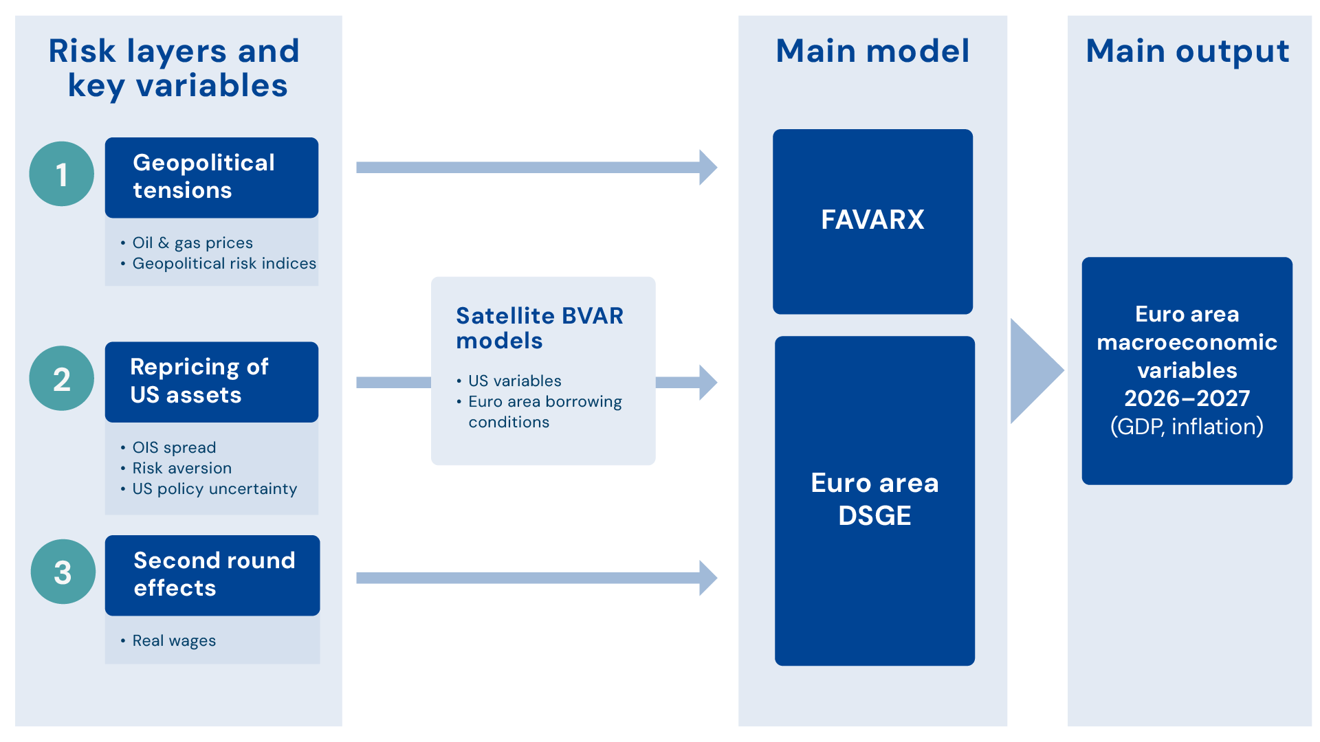
This section describes the modelling approach to the short-term adverse scenario for the euro area. The scenario is constructed by aggregating the estimated impacts of the three risk layers, each modelled using a tailored approach (Figure A6.2). 

Geopolitical tensions and energy prices: non-linear Bayesian FAVAR model

To assess the macroeconomic and financial impact of geopolitical risks and energy shocks on the euro area economy, we employ a non-linear Bayesian FAVAR. The model is described in Capolongo et al. (2026), in the spirit of Brignone et al. (2025). It summarises a large cross-section of macroeconomic and financial variables through 11 latent factors extracted via principal components from a panel covering 10 euro area economies and six other major advanced economies.3 The panel comprises country-level national accounts, prices, trade, financial indicators, and sovereign spreads as well as global indices, including wholesale commodity prices.4 The model is estimated at monthly frequency from January 2000 to June 2026. Results are eventually converted into quarterly frequency.

In a first step, we identify structural shocks using a Cholesky decomposition of the FAVAR. The identified structural shocks are used to calibrate the paths for four variables: wholesale oil and gas prices, an ESM proprietary energy geopolitical risk index, and a euro area geopolitical risk index (following the approach of Caldara and Iacoviello, 2022). The identification strategy imposes the restriction that contemporaneous innovations to observed variables (geopolitical risk indices and energy prices) are not driven by shocks to the remaining macro-financial panel within the same period.  

In a second step, the identified structural shocks enter as exogenous regressors in a non-linear FAVAR with exogenous variables (FAVARX). Each variable is included both in linear and in squared terms. This specification follows the non-linear FAVAR with exogenous variables (FAVARX) framework, extending the methodology of Forni and Gambetti (2024) and Brignone et al. (2025). The linear component captures the standard propagation of each shock, while the squared term captures magnitude-dependent amplification: larger geopolitical or commodity price shocks have a disproportionately stronger impact on the economy than that implied by a linear extrapolation from small shocks. Both stages are estimated with 20,000 posterior draws under a Minnesota prior. 

Based on this framework, we run a conditional forecast under a specific geopolitical scenario: a large initial spike during a single month of the forecast horizon (three standard deviations for the oil shock and four standard deviations for each of the two geopolitical risk shocks), followed by moderate persistence at 0.1 standard deviations for five months, after which no further shocks are imposed. This shock profile captures a sudden, severe geopolitical event with a short-lived tail of elevated risk. The framework compares the resulting conditional forecast with the baseline. It attributes forecast movements to individual shocks by passing each shock through the median vector moving-average impulse-response kernels, thereby combining standard linear propagation with non-linear amplification. 

US asset repricing: BVAR and DSGE models

Spillovers from a sharp repricing of US assets to the euro area are quantified using a combination of models. In the scenario, the repricing is triggered by a sharp rise in US policy uncertainty. Satellite BVARs are used to calibrate the shock, assess its financial and macroeconomic effects in the US, and trace its implications for euro area financial conditions. In a second step, these results are mapped into euro area macroeconomic outcomes using a DSGE framework. 

We assess the macro-financial impact of a rise in policy uncertainty and repricing of US assets with a BVAR model tailored towards US macroeconomic and financial variables. The model comprises the ESM proprietary economic policy uncertainty (EPU) index for the US, the VIX (an option-implied measure of US stock market volatility), the S&P500, the 10-year overnight index swap (OIS) yield, the federal funds rate, the excess bond premium,5 employment, inflation, GDP, consumption, investment, the EUR/USD exchange rate, the Euro Stoxx 600, and the10-year German government bond yield. It is estimated at quarterly frequency starting in Q1 1996 and ending in Q4 2025. The macroeconomic variables are considered in real terms. Based on this model, we run a conditional forecast, conditioning on a path for the EPU, the VIX, the OIS spread, and the excess bond premium to extract the relevant shocks aligned with our narrative. 

We use a separate BVAR to explore implications for euro area borrowing conditions. The variables in the model comprise the US EPU index, the VIX, the excess bond premium for the US, the S&P500, the Euro Stoxx 600, the BBB spread for the euro area, the 10-year German government bond yield, the Euribor, the spread between the lending rate  (non-financial corporations) and the Euribor, and the increase in bank loans to non-financial corporations (deflated). The model is estimated over a slightly shorter period due to data availability constraints for euro area loan data (from Q1 2001 to Q2 2025). A conditional forecast is conducted by conditioning on the paths of US variables derived from the US-focused BVAR.  

The final impact on the euro area economy of both financial and trade channels is obtained by combining the results of two separate simulation exercises: 

  • To assess the macroeconomic implications of financial amplification in the euro area, the resulting paths are fed into a macro-financial euro area DSGE model. Specifically, the paths for credit spreads, the loan spread, credit growth, and interest rates from the euro area markets' BVAR are included in a DSGE model like the one described in Kühl (2018). The model is estimated for the euro area (closed economy) and has an emphasis on financial amplification via an elaborate financial sector.  
  • In addition, to capture the trade channel of transmission to the euro area, we use a three-region DSGE model for an open economy following Cardani et al. (2023). The model features the euro area, the US, and the rest of the world. The model emphasises trade linkages. We run a conditional forecast, conditioning on the US macroeconomic variables that result from the first step BVAR approach. We simulate the impact on the euro area economy while keeping euro area interest rates unchanged. 

Second-round effects on inflation: DSGE approach

The second-round effects on inflation from the rise in energy prices are assessed by using the macro-financial DSGE model for the euro area. A conditional forecast is conducted targeting real wage growth reflecting recent experience. Specifically, it is assumed that workers can negotiate higher wages (around one percentage point higher wage growth than otherwise), which is implemented in the model with a wage mark-up shock. Real wages in the adverse scenario are therefore higher than when abstracting from second-round effects.  

  • 3

    Germany, France, Spain, Italy, Belgium, Finland, Greece, Ireland, the Netherlands, Portugal, the United Kingdom, the US, Canada, Australia, Japan, and Switzerland.

  • 4

    National accounts' variables (GDP and its components, savings, and income) enter as three-period percentage changes (quarter-on-quarter growth rates) with interpolation. Price indices (consumer price index and producer price index), trade, equity indices, and exchange rates enter as month-on-month log differences. Interest rates and sovereign spreads enter in first differences. Oil and gas prices and purchasing managers' indices enter in log levels. Harmonised index of consumer prices measures enters as year-on-year percentage changes. All panel variables are standardised to zero mean and unit variance prior to factor extraction.

  • 5

    The excess bond premium is defined as the component of corporate bond spreads not directly attributable to the expected default risks, as argued in Gilchrist and Zakrajsek (2012). It is a measure of investor sentiment or risk appetite in the corporate bond market.

Figure A6.2

Schematic representation of short-run modelling approach

A6.2.png

Source: ESM

A6.3 Euro area medium- to long-term impact (2028–2035)

This section explains how the short-term adverse scenario is translated into medium- to long-run macroeconomic paths for the euro area. The approach combines evidence on the persistent effects of geopolitical and energy price shocks on productivity and external competitiveness (Section A6.2) with a semi-structural framework. This framework allows us to map these long-run forces into a coherent path for a broader set of macroeconomic variables. 

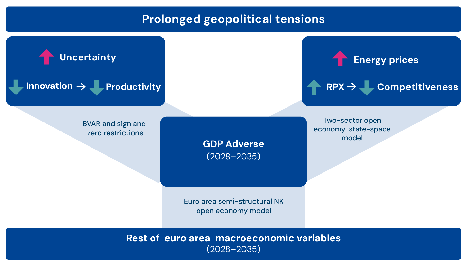
GDP scarring via impaired innovation and export-sector productivity: BVAR

The long-term impact of persistently high geopolitical tensions is identified using a BVAR model and a combination of sign and zero restrictions (Furlanetto et al., 2025; Bratsiotis and Theodoridis, 2022). The model comprises oil and gas prices, geopolitical risk, and the following variables for the euro area: real GDP, inflation, real investment, the relative price of investment, unemployment, the 10-year government bond yield, real wages, investment in research and development as a share of GDP, and total factor productivity. All series are expressed in log levels, except for research and development. The model is estimated using quarterly data from Q1 1999 to Q4 2025, two lags are specified, and a Minnesota-type prior is used to facilitate estimation. To identify the shock of persistently elevated geopolitical tensions, we assume it has zero contemporaneous impact on oil and gas prices, suppresses investment in physical capital and research and development in the short run, and has a permanent impact on total factor productivity and relative price of investment.  

The identified shock captures the narrative that persistent uncertainty discourages corporates from investing in innovation. This harms productivity not only in high-productivity sectors but across the economy. Neither the sign nor the magnitude of the shock's effect on GDP are restricted, letting the data determine the shock's statistical and economic significance for economic activity. Once the shock is identified, its effect on GDP is calculated by conditioning on short- and long-term oil and gas prices and the geopolitical risk profiles presented in Table A6.1 at the end of the document, and the GDP path of the short-term adverse scenario between Q3 2026 and Q4 2027 discussed in the previous section (Section A6.2

The second shock, a deterioration of export-sector productivity, is proxied by a persistent increase in the ratio of export prices to the GDP deflator. In the spirit of Schmitt-Grohe and Uribe (2025) and Gortz et al. (2022), we employ state-space estimation techniques to identify the long-run effect of a permanent increase in the ratio of export prices to the GDP deflator (RPX) on GDP. Given that the RPX for the euro area displays a pronounced downwards sloping trend, we assume that euro area potential supply is driven by two stochastic trends: the (standard) economy-wide trend and an export-specific technological trend. The second technological trend operates within the export sector, expanding at a faster pace than the rest of the economy, consistent with the downward trend in RPX. 

We use a two-sector open-economy DSGE model to identify the shares of the two trends in the economy. The approach followed is like Gortz et al. (2022). The model comprises real GDP growth, real export growth, and RPX growth. It is estimated using quarterly data from Q1 1970 to Q4 2025. Two lags are included to capture cyclical dynamics, and prior information is incorporated in the form of a Minnesota-type prior.6 Finally, the shock is calibrated by gradually unwinding the reduction in the RPX the European Commission foresees over the forecast horizon (European Commission spring 2026 economic forecast).

Taken together, these two channels – innovation and export-sector productivity – drive the medium- to long-term impact on GDP. 

Broader macroeconomic long-term effects: semi-structural model

The medium- to long-run profiles of all variables other than GDP are derived using an open-economy semi-structural NK economic model. Similar to Angelini et al. (2019), a semi-structural macroeconomic NK open-economy model is developed to reconcile the short- and long-term baseline forecasts produced by the European Commission. This also helps assess how alternative assumptions impact the evolution of key series of interest. The model features nominal, real, and financial frictions. The model is estimated with Bayesian maximum likelihood techniques on data from Q1 1995 to Q4 2025.  

  • 6

    To improve the estimation precision of the long-term dynamics we use the Area Wide Model database from the Euro Area Business Cycle Network.

Figure A6.3

Schematic representation of medium-term risks and modelling approach

A6.3.png

Note: RPX is the ratio of export prices to the GDP deflator.
Source: ESM

The semi-structural model generates internally consistent paths for the remaining economic variables conditional on the short-term scenario and long-run restrictions. Given the conditioning assumptions reported in Table A6.1, the short-term (T+1 and T+2) profiles of the economic variables explained in Section A.6.2 and the estimated T+3 to T+10 GDP paths, the model derives conditional forecasts for all other economic variables over theT+3 to T+10 horizon. This ensures that the resulting T+10 scenario extends captures the broader macroeconomic environment in a way that is coherent with the overall adverse narrative. 

A6.4 Euro area countries (2026–2035)

With the euro area medium- to long-run impact of the adverse scenario quantified, the next step is to translate it into country-specific paths. This requires a framework that preserves consistency with the aggregate euro area outlook while allowing for heterogeneity in trade and country-specific exposures, fiscal space, and domestic propagation mechanisms. 

The medium- to long-run profiles of country-specific economic variables are produced using a two-region open-economy semi-structural NK economic model. The model mentioned in the Section A6.3 is further extended into a two-region model comprising the country of interest and the rest of the euro area for each of the euro area member states. From the country's perspective, trade and financial transactions occur with both the rest of the euro area and the rest of the world. 

The two-region structure allows each country’s outlook to be conditioned on the euro area adverse scenario while preserving country-specific transmission mechanisms. In this way, the country scenarios remain consistent with the aggregate euro area narrative but are not constrained to react identically across jurisdictions. 

Country-specific adverse scenarios for T+1 to T+10 profiles are produced in two steps. In the first step, country-specific forecasts are derived conditional on the T+1 to T+10 euro area profiles discussed in Section A6.3. In a second step, the resulting country profiles are reviewed to determine whether country-specific forecasts align with the narrative adopted. For example, persistently higher oil and gas prices should have more severe effects in countries that rely more heavily on fossil fuels and have more limited fiscal space. If this is not the case, then further iterations are undertaken to align the resulting profiles with the judgement of country experts and the euro area risk narrative. This iterative procedure is intended to ensure that the final country paths are aligned with both country-specific expertise and the broader scenario narrative. The result is therefore a set of country projections that is both model-consistent and tailored to the structural characteristics and vulnerabilities of each jurisdiction. 

Strengths and limitations of the framework  

The main strength of the framework is that it combines empirical grounding with structural discipline. Empirical models use data-rich information sets to identify shocks and measure spillovers, while structural models map these shocks into internally consistent macroeconomic outcomes. This design is well suited to adverse scenarios in which non-linear amplification, trade spillovers, and financial frictions all matter. The multi-layered approach also allows the contribution of individual risk layers to be traced and communicated clearly. 

At the same time, the framework also carries limitations. Combining outputs across models with different samples and identifying assumptions introduces aggregation uncertainty. To address this, cross-model consistency and coherence with the scenario narrative are used as organising principles throughout the exercise. Long-run projections are additionally sensitive to assumptions about the persistence of scarring effects. All these considerations suggest the results are best interpreted as one plausible adverse path, to be read alongside the qualitative risk narrative in Chapter 1.  

 
Table A6.1
Key variables for designing the adverse macroeconomic scenario
Key variable Calibration
Short termLong term 

Oil prices 

USD 100/barrel on average in 2026, and USD 87 /barrel in 2027 

USD 87/barrel in 2028–2035 

Gas prices 

€57/megawatt-hour on average in 2026, and €49/megawatt-hour in 2027 

€49/ megawatt-hour in 2028–2035 

Geopolitical risks 

70% and 20% above baseline in 2026 and 2027, respectively 

20% above baseline in 2028-2035 

Energy-related geopolitical risks 

100% and 30% above baseline in 2026 and 2027, respectively 


US 10-year yield- 

OIS spread 

Rising to 60 basis points in 2026 falling to 56 basis points in 2027 


US excess bond premium 

Gradual increase by 50 basis points reached mid-2027 


US policy uncertainty index 

Around 100% above current level by end-2026 


VIX 

Around 60% above baseline by end-2026 


EUR/USD 

Appreciation of the euro by around 2% by end-2027 


US 10-year government bond yields 

Peak increase of around 80 basis points in 2027 


German 10-year government bond yields 

Increase of around 30 basis points by end-2027 

It is kept constant at 30 basis points over baseline 

S&P500 

Almost 20% lower by end-2027 


EURO STOXX 

Almost 30% lower by end-2027 


Source: ESM calculations

A6.6 References

Angelini, E., N. Bokan, K. Christoffel, M. Ciccarelli, and S. Zimic (2019). Introducing ECB-BASE: The blueprint of the new ECB semi-structural model for the euro area. Working Paper Series 2315, European Central Bank.

Bratsiotis, G. and K. Theodoridis (2022). Precautionary liquidity shocks, excess reserves and business cycles. Journal of International Financial Markets, Institutions and Money, 77.

Brignone, D., A. Ferrando, E. Gambetti, and L. Ricci (2025). Geopolitical risk shocks: when size matters. European Central Bank Working Paper.

Caldara, D. and M. Iacoviello (2022). Measuring Geopolitical Risk. American Economic Review.

Capolongo, A., M. Kuehl, and V. Skovorodov (2026). Uncovering nonlinearities: Geopolitical Risk Shocks in the Euro Area. ESM Working Paper, forthcoming.

Cardani, R., P. Pfeiffer, M. Ratto, and L. Vogel (2023). The COVID-19 recession on both sides of the Atlantic: A model-based comparison. European Economic Review, 158, September 2023.

Forni, M., L. Gambetti, N. Maffei-Faccioli, and L. Sala (2024). Nonlinear transmission of financial shocks: some new evidence. Journal of Money, Credit and Banking.

Furlanetto, F., A. Lepetit, A. Robstad, J. Rubio-Ramirez, and P. Ulvedal (2025). Estimating Hysteresis Effects. American Economic Journal: Macroeconomics, 17(1), p. 35-70.

Gilchrist, S. and E. Zakrajšek (2012). Credit spreads and business cycle fluctuations. American Economic Review 102.

Gortz, C., K. Theodoridis, and C. Thoenissen (2022). The Anatomy of Small Open Economy Trends. CAMA Working Papers 2022-06.

Kühl, M. (2018). The Effects of Government Bond Purchases on Leverage Constraints of Banks and Non-Financial Firms. International Journal of Central Banking, 14(4).

Schmitt-Grohe, S. and M. Uribe (2025). The Effects of Transitory, Permanent, and Anticipated U.S. Import Tariff Shocks. NBER, 33997. 

A7 Constructing the baseline and adverse fiscal scenarios

A7.1 Objectives

This note describes the methodology used to construct the fiscal scenarios presented in Chapter 1. These scenarios are designed to assess the fiscal implications of the adverse macroeconomic scenarios specified in Section 1.4 of Chapter 1

This note also explains the approach used to estimate fiscal adjustment needs under the economic governance framework of the European Union (EU). In this context, the scenarios serve to gauge the scale of policy effort that may be required to place public debt on a plausibly downward trajectory or to ensure that it remains at prudent levels. 

A7.2 Baseline scenario based on the European Commission framework with defence spending

The baseline scenario constitutes the central path for the analysis and serves as the benchmark for assessing the adverse scenario. In the short term (2026–2027), the baseline fiscal scenario is aligned with the European Commission’s 2026 spring economic forecast (published on 21 May 2026). Beyond the short-term horizon, projections are extended using the European Commission's methodology underpinning the Debt Sustainability Monitor (European Commission, 2026). 

This approach breaks down the primary fiscal balance into three components: 

  1. the structural primary balance net of ageing costs, which remains constant at its value forecast for T+1, while ageing-related expenditure covering pensions, healthcare, long-term care, and education enter as projected in the joint European Commission-Council of the EU 2024 Ageing Report (as well as property income from government assets); 
  2. the cyclical component, which is determined by the output gap and country-specific budgetary semi-elasticities; and 
  3. one-off and other temporary measures, which are set to zero beyond T+2, in line with a no-policy-change approach.  

Under the baseline scenario, interest rates follow the same methodological approach as the European Commission. For 2026 and 2027, market interest rates are computed using the same reference period of the European Commission spring 2026 economic forecast. Interest rate projections then follow the European Commission's methodology underpinning the Debt Sustainability Monitor (European Commission, 2026) which interpolates between market spot rates and 10Y10Y forward rates.

A7.3 Adverse scenario

The ESM’s adverse fiscal scenario builds on the adverse macroeconomic scenario described in Chapter 1 and incorporates the effects of governments’ military spending commitments. To reflect the sizeable expenditure pressures stemming from countries’ commitments to raise defence spending, the structural primary balance net of ageing costs is adjusted to include additional military expenditure sufficient for each country to reach the North Atlantic Treaty Organisation (NATO) target of 3.5% of gross domestic product (GDP) by 2035. In effect, the scenario treats the gap to the NATO target in the same way as ageing costs, namely as spending pressures that worsen fiscal balances if no other policy changes take place. 

The military expenditure trajectory is based on the information provided in the European Commission’s 2026 spring package, which includes expenditure plans up to 2026. Using the 2026 level of military expenditure as the starting point, additional increases are assumed from 2027 onwards. The trajectory is calibrated to fully utilise the flexibility provided under the national escape clause until 2028, allowing defence expenditure to increase by up to 1.5 percentage points of GDP without breaching the EU fiscal rules. 

Thereafter, military expenditure is assumed to increase linearly until reaching the NATO benchmark of 3.5% of GDP by 2035. The benchmark applies to all euro area countries. For non-NATO euro area countries, the 3.5% of GDP benchmark is an analytical assumption rather than a formal policy commitment.  

Structural primary expenditures are assumed to grow in line with baseline nominal potential GDP growth. This therefore constitutes a no-policy-change scenario, in which the government maintains baseline policies without adjusting expenditure in response to the weaker macroeconomic environment. The change in the structural primary balance (SPB) under the adverse scenario is therefore given by  

\[ \Delta SPB_t = \frac{\text{Primary Expenditure}}{\text{GDP}} \cdot \left( g_t^{\text{Pot, Adverse}} - g_t^{\text{Pot, Baseline}} \right) \]

where \[ g_t^{\mathrm{Pot}} \] denotes nominal potential GDP growth. Lower potential growth in the adverse scenario therefore leads to a mechanical deterioration in the structural primary balance at unchanged policies. 

The cyclical component of the primary balance adjusts to reflect the updated output gap estimates derived from the adverse macroeconomic scenario. Compared to the baseline, the output gap closes more gradually under the adverse,7 thereby prolonging the cyclical drag on public finances. 

The overall primary balance is then obtained by adding ageing-related expenditure and property income on government assets. Both components are assumed to evolve in line with the baseline scenario. Taken together, all these factors result in persistently weaker primary balances under the adverse scenario compared to the baseline scenario. 

Finally, interest rate projections in the adverse scenario reflect the impact of the different risk layers on government bond yields (Section 1.4 of Chapter 1). In the short term (2026–2027), deviations of German government bond yields from the baseline path are derived from the modelling of the adverse macroeconomic scenario (Section 1.4 of Chapter 1 and Annex A6). For other euro area countries, sovereign bond spreads vis‑à‑vis German government bond yields are estimated using a simplified structural scenario analysis tool (cf. Antolin-Diaz et al., 2021). This tool relies on a monthly panel regression model linking sovereign spreads to macroeconomic, fiscal, monetary, and global financial variables that capture credit risk, liquidity risk, and overall risk aversion. As the effects of external shocks gradually fade, sovereign spreads are estimated considering the evolution of country‑specific fiscal variables. 

A7.4 Fiscal adjustment under the European economic governance framework

Assumptions underlying fiscal adjustment paths

The analysis of adjustment needs under the European economic governance framework focuses on the fiscal effort required in the second round of medium-term fiscal-structural plans. The second round starts after 2028, to ensure compliance with the fiscal rules while accommodating the increase in military spending (Council of the European Union, 2024). 

In the current round of medium-term fiscal-structural plans (2027–2028), we assume that countries increase their net expenditure in line with Council recommendations, taking full advantage of national escape clauses. Thereafter, a debt sustainability analysis is conducted for all countries, assuming that each country requests a seven-year adjustment period under the EU fiscal framework as this is the permissible extended period available to Member States. The adjustment needs are determined by compliance with the debt sustainability criterion, ensuring that public debt is placed on a plausibly downward trajectory. Given the stylised nature of the exercise, however, compliance with the debt sustainability safeguard, which requires a minimum reduction in the debt ratio for countries with public debt above 60% of GDP, and the deficit resilience safeguard, which requires maintaining a fiscal buffer below the 3% of GDP deficit reference value, are not imposed as additional criteria.  

This approach explicitly accounts for the additional fiscal adjustment required to accommodate long-term spending pressures from defence and ageing, while also reflecting the impact of weaker macroeconomic performance on fiscal positions relative to the baseline. 

Decomposition of fiscal adjustment needs

This section clarifies our definition of fiscal adjustment and provides a decomposition to identify the adjustment needed to offset the deterioration in fiscal outcomes arising from adverse macroeconomic conditions, demographic pressures, and military expenditure commitments.  

Let \[ \Delta SPB_t^{\mathrm{X,Scen}} \] denote the annual change in the structural primary balance in year t, where X ∈ {Adj,NPC} refers to the path of the structural primary balance consistent with the fiscal rules and no-policy-change, while Scen ∈ {Baseline,Adverse} denotes the macroeconomic scenario.

We define the adjustment required under the fiscal rules relative to the no-policy-change scenario over the period 2026–2035 as:

\[ \mathrm{Adjustment}^{\mathrm{Scen}} = \sum_{t=2026}^{2035} \left( \Delta SPB_t^{\mathrm{Adj,Scen}} - \Delta SPB_t^{\mathrm{NPC,Scen}} \right) . \]

Under the no-policy-change scenario, the structural primary balance deteriorates mechanically because increases in military expenditure and ageing-related costs are not offset by policy measures. Achieving the target fiscal position implied by the fiscal rule requires discretionary measures to compensate for these expenditures. This distinction is analytically important. If adjustment was measured excluding these expenditures, we would understate the actual consolidation effort required to comply with the fiscal framework.  

Denoting by \[ \check{SPB} \] the structural primary balance excluding military expenditures and cost of ageing, the adjustment can be decomposed as:

\[ \mathrm{Adjustment}^{\mathrm{Scen}} = \sum_{t=2026}^{2035} \left( \Delta SPB_t^{\mathrm{Adj,Scen}} - \Delta \check{SPB}_t^{\mathrm{NPC,Scen}} \right) + \sum_{t=2026}^{2035} \Delta \mathrm{Military}_t + \sum_{t=2026}^{2035} \Delta \mathrm{CoA g}_t . \]

This decomposition isolates the contribution of military expenditure and ageing costs to total adjustment requirements. 

Under the adverse scenario, the first term can be further decomposed as: 

\[ \sum_{t=2026}^{2035} \left( \Delta SPB_t^{\mathrm{Adj,Adverse}} - \Delta \check{SPB}_t^{\mathrm{NPC,Baseline}} \right) + \sum_{t=2026}^{2035} \left( \Delta \check{SPB}_t^{\mathrm{NPC,Baseline}} - \Delta \check{SPB}_t^{\mathrm{NPC,Adverse}} \right) . \]

The first term captures the distance between the target structural position under the rule at the end of the adjustment horizon and the corresponding structural position under no-policy- change, excluding military expenditure and the cost of ageing. The second term singles out the additional consolidation required solely to offset the deterioration in fiscal outcomes caused by weaker macroeconomic conditions under unchanged policies. 

The maximum realised historical adjustment is calculated as the largest improvement in the cyclically adjusted primary balance (CAPB) recorded during a qualifying fiscal consolidation episode over the period 1995–2025. The analysis starts in 1995, as CAPB data are not available for a sufficiently large number of countries before that date. A qualifying fiscal consolidation episode is defined as a period in which the CAPB improves in each year of the episode and cumulatively by at least two percentage points of GDP over two years or by at least three percentage points of GDP over three or more years (Callegari et al., 2025). The consolidation episodes for Greece, Portugal and Ireland during financial assistance programmes are excluded. 


A7.5 References

Antolín-Díaz, J., I. Petrella, and J. F. Rubio-Ramírez (2021). Structural scenario analysis with SVARs. Journal of Monetary Economics, 117, 798–815. 

Callegari, G., V. Michou, K.V., Slawinska, D.K., Žigraiová, and D., & F. Tomasone, F. (2025). Spending composition and fiscal consolidation: Enhancing resilience in the face of economic shocks. ESM Working Paper 73.

Council of the European Union. (2024). Regulation of the European Parliament and of the Council on the effective coordination of economic policies and on multilateral budgetary surveillance and repealing Council Regulation (EC) No 1466/97. 

European Commission (2024). 2024 Ageing report: Economic and budgetary projections for the EU Member States (2022–2070), European Economy Institutional Paper No. 279.

European Commission. (2026). Debt Sustainability Monitor 2025. 

European Commission. (2026). European economic forecast: Spring 2026.

European Commission (2026). 2026 European Semester: Spring package.

A8 Methodological notes on fiscal space scores

This annex presents the framework used in Chapter 1 to assess fiscal space across euro area countries. Fiscal space is measured using a composite indicator of projections of four core fiscal variables. The objective of this indicator is to provide a transparent and internally consistent measure of countries’ relative fiscal space under both the baseline and the adverse macroeconomic scenario. The proposed framework reflects ongoing work and is intended for cross-country comparison in the euro area under different scenarios. 

A8.1 Fiscal space and its determinants

Fiscal space reflects the interplay of several dimensions of a government's fiscal position. Fiscal space is understood as the capacity of a government to adjust spending or taxes while preserving sound public finance. It is inherently multi-dimensional, as it encompasses considerations related to debt sustainability, fiscal position, and flexibility (Kose, Kurlat, Ohnsorge, and Sugawara, 2022; IMF, 2018). To capture these dimensions in a transparent and tractable manner, the analysis focuses on four indicators, each capturing a distinct and complementary dimension of fiscal space. 

  • The government debt-to-revenue ratio measures the burden of public debt relative to the government’s capacity to generate income. Debt measured relative to the tax base provides an informative measure of fiscal space because it links public debt to the resources available for servicing and managing that debt (Aizenman, Jinjarak, Nguyen, and Park, 2019). 
  • The budget balance, measured as the overall general government balance as a share of gross domestic product (GDP), reflects the underlying fiscal position and the degree to which a government is adding to or reducing its debt stock.  
  • Fiscal flexibility, defined as the difference between total revenue and rigid expenditure expressed as a share of total revenue, captures the proportion of government revenues that can be actively deployed. Rigid expenditures, such as on pensions, interest payments, and compensation of employees, are difficult to adjust in the short run; a government with limited flexibility has little room to manoeuvre even if its overall fiscal position appears adequate.  
  • The interest-growth differential is measured in nominal terms and captures the dynamic of public debt accumulation by comparing the cost of borrowing to the pace of economic growth.  

A8.2 Technical calculations

All indicators are standardised using z-scores. For each of the four fiscal indicators, z-scores are computed separately using the cross-country distribution of the indicator across euro area countries in the 2028 baseline scenario as the reference benchmark. The 2028 values are based on ESM scenario calculations, anchored in European Commission projections. The 2028 horizon is used because the fiscal impact of the adverse shock materialises with a lag, once the initial inflationary pressures fade: as inflation normalises, the loss in potential GDP translates into a deterioration in the structural balance (see Annex A7 for further details). 

Standardisation allows comparing the relative ranking of countries along the four dimensions of fiscal space. Prior to the calculation, each variable is sign-adjusted so that higher values consistently reflect an improvement in fiscal space. Formally, for each indicator i and country c, the standardised score is computed as

\[ z_{i,c} = \frac{(x_{i,c} - \mu_i)}{\sigma_i} \]

where xi,c denotes the raw value of the indicator based on 2028 baseline projection values, and 𝜇i and 𝜎i are the cross-country mean and standard deviation in the 2028 baseline scenario. For each country, the z-score measures the distance of the indicator from the baseline cross-country distribution, expressed in standard deviation units.8 A value of zero indicates that the country is at the euro area average, while positive (negative) values indicate a stronger (weaker) position relative to the average.


In the adverse scenario, the z-score compares country projections under the adverse scenario to those under the baseline. Specifically: 

\[ z_{i,c}^{adv} = \frac{(x_{i,c}^{adv} - \mu_i^{baseline})}{\sigma_i^{baseline}} \]

Keeping the baseline benchmark fixed allows changes between the baseline and adverse scenarios to be interpreted as changes in fiscal space relative to the same reference distribution. A deterioration in the underlying fiscal indicators under the adverse scenario is therefore reflected in lower z-scores. This reflects the intuitive and empirically supported result that fiscal space contracts under adverse conditions (Ghosh, 2013). 

The composite fiscal space score is then calculated as the simple average of the four standardised indicators:

\[ FS_c = \frac{1}{4} \sum_{i=1}^{4} z_{i,c} \]

All indicators are equally weighted. For ease of interpretation, the composite fiscal space score is additionally mapped into a 0-100 index using the cumulative normal distribution. Specifically, the index is defined as 100 × ϕ(z), where ϕ denotes the standard normal cumulative distribution function. Under this transformation, a value of 50 corresponds to the euro area average, while higher (lower) values indicate more (less) fiscal space. This transformation is monotonic and does not affect country rankings or underlying results.

A8.3 Classification and interpretation

For ease of interpretation, countries are grouped into three categories based on their composite score, as shown in Table A8.1. For presentation purposes, results are expressed using the 0-100 fiscal space index. The classification thresholds correspond directly to the underlying z-score cutoffs: countries with an index value of 16 or below are classified as having limited fiscal space, those with values between 16 and 84 as having some fiscal space, and those above 84 as having ample fiscal space. These thresholds correspond to z-scores of −1 and +1, respectively.9

The baseline results show each country’s position relative to the euro area average under baseline conditions (in T+3). The adverse results show how the same country performs under stress in T+3, still evaluated against the baseline benchmark. This allows differences between scenarios to be interpreted directly as deterioration or improvement in fiscal space relative to baseline conditions. 

A8.4 Caveats

Being a relative measure of fiscal space, the composite indicator abstracts from common factors that determine fiscal space in an absolute sense, such as investor risk appetite, global financial conditions, and euro area monetary policy. Furthermore, the interpretation of z-scores assumes that the underlying distribution of indicators is reasonably well-behaved, such that standard deviation is an informative measure of dispersion. 

The relationship between fiscal space and medium-term adjustment needs is presented in Figure A8.1 as a validation exercise for the composite indicator. Conceptually, countries that already require larger fiscal adjustments should have more limited fiscal space as weaker fiscal positions constrain their ability to absorb shocks or sustain current policies. Furthermore, while adjustment needs are sometimes considered a potential component of fiscal space measures, the strong negative correlation observed in the data suggests that the current indicator already captures this dimension indirectly. Countries assessed as having more limited fiscal space tend, in practice, to face larger adjustment requirements. This suggests that the fiscal space measure proposed here reflects economically meaningful constraints. 

 
  • 7

    The closure of the output gap is country specific and driven by a model-based quantification of the adverse scenario. Nevertheless, it is assumed to close by T+10 at the latest.

  • 8

    To limit the influence of extreme observations, the reference distribution is winsorised, meaning that values below the 5th percentile and above the 95th percentile are capped before computing the mean and standard deviation; these baseline parameters are then kept fixed across scenarios.

  • 9

    Values at least one standard deviation below the mean (z ≤ −1) are classified as weaker fiscal space (red), values within one standard deviation of the mean (−1 < z ≤ 1) as average fiscal space (orange), and values above one standard deviation (z > 1) as stronger fiscal space (green).

Table A8.1
Grouping of countries based on fiscal space indicators
CountryBaseline indexAdverse index
Ireland
97 dotHigh
87 dotHigh
Cyprus
89 dotHigh
73 dotMedium
Malta
87 dotHigh
64 dotMedium
Netherlands
87 dotHigh
76 dotMedium
Luxembourg
82 dotMedium
70 dotMedium
Croatia
67dotMedium
44dotMedium
Germany
59dotMedium
43dotMedium
Lithuania
54dotMedium
14dotLow
Slovenia
48dotMedium
23dotMedium
Portugal
44dotMedium
22dotMedium
Estonia
39dotMedium
26dotMedium
Bulgaria
38dotMedium
15dotLow
Greece
35dotMedium
18dotMedium
Austria
34dotMedium
20dotMedium
Spain
32dotMedium
10dotLow
Latvia
28dotMedium
14dotLow
Slovakia
28dotMedium
13dotLow
Belgium
26dotMedium
10dotLow
Finland
25dotMedium
15dotLow
France
14dotLow
5dotLow
Italy
8dotLow
2dotLow
Notes: Countries are classified into three groups: limited (index ≤ 16), some (16 < index ≤ 84), and ample fiscal space (index > 84), corresponding to z-score thresholds of −1 and +1, and are shown using red, orange and green, respectively. The adverse scenario is evaluated against the same baseline benchmark to ensure comparability. Source: ESM calculation based on European Commission’s spring 2026 economic forecast data, Eurostat data, European Commission's spring 2026 package data and the 2024 Ageing Report
 

Figure A8.1

Fiscal space and adjustment needs: baseline and adverse scenarios

a)
Baseline (baseline benchmark)
(x-axis: in percentage points of GDP, y-axis: index)
b)
Adverse (baseline benchmark)
(x-axis: in percentage points of GDP, y-axis: index)

Notes: Fiscal space is measured using the composite fiscal space index (0-100 scale, derived from the underlying z-scores), where higher values indicate more fiscal space and 50 corresponds to the euro area average, while adjustment needs correspond to the required annual fiscal effort over 2026–2035. The dashed line shows the fitted linear trend. In both panels, fiscal space is evaluated relative to the 2028 baseline cross-country distribution, ensuring comparability across scenarios.
Source: ESM calculation based on European Commission’s spring 2026 economic forecast data, Eurostat data, European Commission's spring 2026 package data and the 2024 Ageing Report

A8.5 Detailed fiscal space results

This section presents the detailed country-level results underlying the fiscal space assessment. It reports the values of the four underlying indicators – debt-to-revenue, budget balance, fiscal flexibility, and the interest-growth differential – as well as the resulting composite fiscal space scores for each euro area country. While the main text presents the 0-100 fiscal space index for ease of interpretation, this section reports the underlying z-scores relative to the 2028 baseline distribution. Results are shown for both the baseline (Table A8.2) and adverse (Table A8.3) scenarios, allowing a direct comparison of fiscal positions under normal conditions and under stress, and its underlying factors. For example, high debt levels and persistent fiscal deficits are the main factors limiting fiscal space in France, whereas Greece’s steadily improving budget balance enables it to gain some fiscal space despite having a less favourable debt-to-revenue ratio than France in the baseline scenario. Furthermore, lower growth and higher interest rates further constrain fiscal space for most countries under the adverse scenario.  

As robustness checks, fiscal-space scores are also standardised using a historically anchored euro area benchmark for 2002–2024, and classifications are assessed under alternative threshold values. The main patterns remain broadly unchanged, although higher thresholds concentrate more countries in the intermediate category, while lower thresholds produce greater dispersion across high and low fiscal-space groups. 

 
Table A8.2
Grouping of countries based on fiscal space indicators under baseline
CountryDebt to revenueBudget balance
(% GDP)
Fiscal flexibilityInterest-growthBaseline
composite
Austria
-0.20dotSome
-0.67dotSome
-0.38dotSome
-0.38dotSome
-0.41dotSome
Belgium
-1.30dotLimited
-1.16dotLimited
0.08dotSome
-0.20dotSome
-0.65dotSome
Bulgaria
1.07dotAmple
-0.50dotSome
-1.73dotLimited
-0.07dotSome
-0.31dotSome
Croatia
0.76dotSome
0.03dotSome
0.28dotSome
0.72dotSome
0.45dotSome
Cyprus
1.16dotAmple
2.57dotAmple
0.37dotSome
0.78dotSome
1.22dotAmple
Estonia
1.29dotAmple
-0.91dotSome
-0.41dotSome
-1.10dotLimited
-0.28dotSome
Finland
-0.39dotSome
-0.74dotSome
-1.19dotLimited
-0.35dotSome
-0.67dotSome
France
-1.38dotLimited
-1.37dotLimited
-0.58dotSome
-0.98dotSome
-1.08dotLimited
Germany
0.09dotSome
-0.67dotSome
1.78dotAmple
-0.33dotSome
0.22dotSome
Greece
-1.86dotLimited
1.48dotAmple
-0.36dotSome
-0.79dotSome
-0.38dotSome
Ireland
0.64dotSome
1.99dotAmple
2.18dotAmple
2.52dotAmple
1.83dotAmple
Italy
-2.31dotLimited
-0.14dotSome
-1.06dotLimited
-2.16dotLimited
-1.41dotLimited
Latvia
0.40dotSome
-0.78dotSome
-0.67dotSome
-1.24dotLimited
-0.57dotSome
Lithuania
0.52dotSome
-0.08dotSome
-0.32dotSome
0.24dotSome
0.09dotSome
Luxembourg
1.69dotAmple
0.82dotSome
0.74dotSome
0.40dotSome
0.91dotSome
Malta
0.61dotSome
0.57dotSome
0.87dotSome
2.55dotAmple
1.15dotAmple
Netherlands
0.87dotSome
0.51dotSome
2.99dotAmple
0.06dotSome
1.11dotAmple
Portugal
-0.69dotSome
1.13dotAmple
-0.89dotSome
-0.18dotSome
-0.16dotSome
Slovakia
-0.12dotSome
-1.33dotLimited
-0.27dotSome
-0.56dotSome
-0.57dotSome
Slovenia
0.26dotSome
-0.49dotSome
-0.45dotSome
0.48dotSome
-0.05dotSome
Spain
-1.16dotLimited
0.27dotSome
-0.71dotSome
-0.28dotSome
-0.47dotSome
Notes: Fiscal space is measured as the simple average of four sign-adjusted indicators, expressed as z-scores so that higher values indicate more fiscal space. Countries are grouped into three categories: limited, some, and ample fiscal space, with colours aligned with the corresponding charts using red, orange and green. Red denotes below-average fiscal space (z ≤ -1), orange indicates a position close to the euro area average (-1 < z ≤ 1), and green reflects above-average fiscal space (z > 1). Source: ESM calculations based on European Commission’s spring 2026 economic forecast data, Eurostat data, European Commission's spring 2026 package data and the 2024 Ageing Report
 
Table A8.3
Grouping of countries based on fiscal space indicators under adverse
CountryDebt to revenueBudget balance
(% GDP)
Fiscal flexibilityInterest-growthAdverse
composite
Austria
-0.30dotSome
-1.36dotLimited
-0.67dotSome
-1.05dotLimited
-0.84dotSome
Belgium
-1.55dotLimited
-1.86dotLimited
-0.25dotSome
-1.43dotLimited
-1.27dotLimited
Bulgaria
1.01dotAmple
-1.04dotLimited
-2.07dotLimited
-2.06dotLimited
-1.04dotLimited
Croatia
0.65dotSome
-0.66dotSome
-0.02dotSome
-0.60dotSome
-0.16dotSome
Cyprus
0.99dotSome
1.79dotAmple
-0.01dotSome
-0.27dotSome
0.62dotSome
Estonia
1.41dotAmple
-0.67dotSome
-0.26dotSome
-3.00dotLimited
-0.63dotSome
Finland
-0.47dotSome
-1.09dotLimited
-1.34dotLimited
-1.31dotLimited
-1.05dotLimited
France
-1.62dotLimited
-2.16dotLimited
-0.94dotSome
-1.69dotLimited
-1.60dotLimited
Germany
0.00dotSome
-1.16dotLimited
1.58dotAmple
-1.16dotLimited
-0.18dotSome
Greece
-2.04dotLimited
0.74dotSome
-0.70dotSome
-1.69dotLimited
-0.92dotSome
Ireland
0.28dotSome
1.17dotAmple
1.53dotAmple
1.48dotAmple
1.12dotAmple
Italy
-2.58dotLimited
-1.05dotLimited
-1.52dotLimited
-2.88dotLimited
-2.01dotLimited
Latvia
0.44dotSome
-1.06dotLimited
-0.77dotSome
-3.00dotLimited
-1.10dotLimited
Lithuania
0.19dotSome
-1.20dotLimited
-0.95dotSome
-2.31dotLimited
-1.07dotLimited
Luxembourg
1.66dotAmple
0.40dotSome
0.56dotSome
-0.53dotSome
0.52dotSome
Malta
0.32dotSome
-0.45dotSome
0.29dotSome
1.31dotAmple
0.37dotSome
Netherlands
0.78dotSome
0.05dotSome
2.82dotAmple
-0.84dotSome
0.70dotSome
Portugal
-0.95dotSome
0.20dotSome
-1.42dotLimited
-0.87dotSome
-0.76dotSome
Slovakia
-0.17dotSome
-1.93dotLimited
-0.55dotSome
-1.83dotLimited
-1.12dotLimited
Slovenia
0.05dotSome
-1.46dotLimited
-0.94dotSome
-0.65dotSome
-0.75dotSome
Spain
-1.54dotLimited
-0.73dotSome
-1.27dotLimited
-1.61dotLimited
-1.29dotLimited
Notes: Fiscal space is measured as the simple average of four sign-adjusted, expressed as z-scores so that higher values indicate more fiscal space. Countries are grouped into three categories: limited, some, and ample fiscal space, with colours aligned with the corresponding charts using red, orange and green. Red denotes below-average fiscal space (z ≤ -1), orange indicates a position close to the euro area average (-1 < z ≤ 1), and green reflects above-average fiscal space (z > 1). Source: ESM calculations based on European Commission’s spring 2026 economic forecast data, Eurostat data, European Commission's spring 2026 package data and the 2024 Ageing Report

A8.6 References

Aizenman, J., Y. Jinjarak, H.T. Nguyen, and D. Park (2019). Fiscal space and government-spending and tax-rate cyclicality patterns: A cross-country comparison, 1960–2016. Journal of Macroeconomics, 229-252.

European Commission (2024). 2024 Ageing report: Economic and budgetary projections for the EU Member States (2022–2070), European Economy Institutional Paper No. 279.

European Commission. (2026). European economic forecast: Spring 2026. 

European Commission (2026). 2026 European Semester: Spring package.

Ghosh, A. R. (2013). Fiscal fatigue, fiscal space and debt sustainability in advanced economies. The Economic Journal.

IMF. (2018). Assessing Fiscal Space: An Update and Stocktaking. Washington, DC: IMF Policy Paper.

Kose, A. M., S. Kurlat, F. Ohnsorge, and N. Sugawara (2022). A cross-country database of fiscal space. Journal of International Money and Finance.